来自北卡罗来纳大学BIOL222的艺术

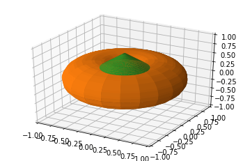
# get library for 3d plotting
from mpl_toolkits.mplot3d import Axes3D

# make a pumpkin :)
rho = np.linspace(0, 3 * np.pi, 32)
theta, phi = np.meshgrid(rho, rho)
r, R = 0.5, 0.5
X = (R + r * np.cos(phi)) * np.cos(theta)
Y = (R + r * np.cos(phi)) * np.sin(theta)
Z = r * np.sin(phi)

# make the stem
theta1 = np.linspace(0, 2 * np.pi, 90)
r1 = np.linspace(0, 3, 50)
T1, R1 = np.meshgrid(theta1, r1)
X1 = R1 * 0.5 * np.sin(T1)
Y1 = R1 * 0.5 * np.cos(T1)
Z1 = -(np.sqrt(X1**2 + Y1**2) - 0.7)
Z1[Z1 < 0.3] = np.nan
Z1[Z1 > 0.7] = np.nan

# Display the pumpkin & stem
fig = plt.figure()
ax = fig.gca(projection="3d")
ax.set_xlim3d(-1, 1)
ax.set_ylim3d(-1, 1)
ax.set_zlim3d(-1, 1)
ax.plot_surface(X, Y, Z, color="tab:orange", rstride=1, cstride=1)
ax.plot_surface(X1, Y1, Z1, color="tab:green", rstride=1, cstride=1)
plt.show()

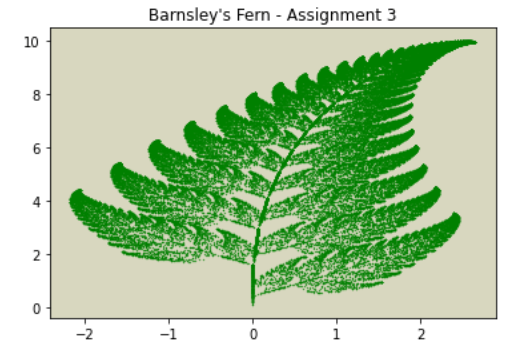
import numpy as np
import matplotlib.pyplot as plt

# Barnsley's Fern - Fractal; en.wikipedia.org/wiki/Barnsley_…


# functions for each part of fern:
# stem
def stem(x, y):
    return (0, 0.16 * y)


# smaller leaflets
def smallLeaf(x, y):
    return (0.85 * x + 0.04 * y, -0.04 * x + 0.85 * y + 1.6)


# large left leaflets
def leftLarge(x, y):
    return (0.2 * x - 0.26 * y, 0.23 * x + 0.22 * y + 1.6)


# large right leftlets
def rightLarge(x, y):
    return (-0.15 * x + 0.28 * y, 0.26 * x + 0.24 * y + 0.44)


componentFunctions = [stem, smallLeaf, leftLarge, rightLarge]

# number of data points and frequencies for parts of fern generated:
# lists with all 75000 datapoints
datapoints = 75000
x, y = 0, 0
datapointsX = []
datapointsY = []
# For 75,000 datapoints
for n in range(datapoints):
    FrequencyFunction = np.random.choice(componentFunctions, p=[0.01, 0.85, 0.07, 0.07])
    x, y = FrequencyFunction(x, y)
    datapointsX.append(x)
    datapointsY.append(y)

# Scatter plot & scaled down to 0.1 to show more definition:
plt.scatter(datapointsX, datapointsY, s=0.1, color="g")
# Title of Figure
plt.title("Barnsley's Fern - Assignment 3")
# Changing background color
ax = plt.axes()
ax.set_facecolor("#d8d7bf")

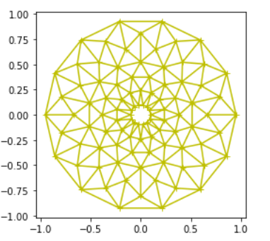
import matplotlib.pyplot as plt
from matplotlib.tri import Triangulation
from matplotlib.patches import Polygon
import numpy as np


# I found this sample code online and manipulated it to make the art piece!
# was interested in because it combined what we used for functions as well as what we used for plotting with (x,y)
def update_polygon(tri):
    if tri == -1:
        points = [0, 0, 0]
    else:
        points = triang.triangles[tri]
    xs = triang.x[points]
    ys = triang.y[points]
    polygon.set_xy(np.column_stack([xs, ys]))


def on_mouse_move(event):
    if event.inaxes is None:
        tri = -1
    else:
        tri = trifinder(event.xdata, event.ydata)
    update_polygon(tri)
    ax.set_title(f"In triangle {tri}")
    event.canvas.draw()


# this is the info that creates the angles
n_angles = 14
n_radii = 7
min_radius = 0.1  # the radius of the middle circle can move with this variable
radii = np.linspace(min_radius, 0.95, n_radii)
angles = np.linspace(0, 2 * np.pi, n_angles, endpoint=False)
angles = np.repeat(angles[..., np.newaxis], n_radii, axis=1)
angles[:, 1::2] += np.pi / n_angles
x = (radii * np.cos(angles)).flatten()
y = (radii * np.sin(angles)).flatten()
triang = Triangulation(x, y)
triang.set_mask(
    np.hypot(x[triang.triangles].mean(axis=1), y[triang.triangles].mean(axis=1))
    < min_radius
)

trifinder = triang.get_trifinder()

fig, ax = plt.subplots(subplot_kw={"aspect": "equal"})
ax.triplot(
    triang, "y+-"
)  # made the color of the plot yellow and there are "+" for the data points but you can't really see them because of the lines crossing
polygon = Polygon([[0, 0], [0, 0]], facecolor="y")
update_polygon(-1)
ax.add_patch(polygon)
fig.canvas.mpl_connect("motion_notify_event", on_mouse_move)
plt.show()

import numpy as np
import matplotlib.pyplot as plt

plt.axis("off")

# head
xhead = np.arange(-50, 50, 0.1)
yhead = -0.007 * (xhead * xhead) + 100

plt.plot(xhead, yhead, "darkorange")

# outer ears
xearL = np.arange(-45.8, -9, 0.1)
yearL = -0.08 * (xearL * xearL) - 4 * xearL + 70

xearR = np.arange(9, 45.8, 0.1)
yearR = -0.08 * (xearR * xearR) + 4 * xearR + 70

plt.plot(xearL, yearL, "black")
plt.plot(xearR, yearR, "black")

# inner ears
xinL = np.arange(-41.1, -13.7, 0.1)
yinL = -0.08 * (xinL * xinL) - 4 * xinL + 59

xinR = np.arange(13.7, 41.1, 0.1)
yinR = -0.08 * (xinR * xinR) + 4 * xinR + 59

plt.plot(xinL, yinL, "salmon")
plt.plot(xinR, yinR, "salmon")

# bottom of face
xfaceL = np.arange(-49.6, -14, 0.1)
xfaceR = np.arange(14, 49.3, 0.1)
xfaceM = np.arange(-14, 14, 0.1)

plt.plot(xfaceL, abs(xfaceL), "darkorange")
plt.plot(xfaceR, abs(xfaceR), "darkorange")
plt.plot(xfaceM, abs(xfaceM), "black")

# nose
xnose = np.arange(-14, 14, 0.1)
ynose = -0.03 * (xnose * xnose) + 20

plt.plot(xnose, ynose, "black")

# whiskers
xwhiskR = [50, 70, 55, 70, 55, 70, 49.3]
xwhiskL = [-50, -70, -55, -70, -55, -70, -49.3]
ywhisk = [82.6, 85, 70, 65, 60, 45, 49.3]

plt.plot(xwhiskR, ywhisk, "darkorange")
plt.plot(xwhiskL, ywhisk, "darkorange")

# eyes
plt.plot(20, 60, color="black", marker="o", markersize=15)
plt.plot(-20, 60, color="black", marker="o", markersize=15)

plt.plot(22, 62, color="white", marker="o", markersize=6)
plt.plot(-18, 62, color="white", marker="o", markersize=6)