博客 - 初等元胞自动机 - 科学 Python 博客

元胞自动机是离散模型，通常在网格上，随着时间演化。每个网格单元都有一个有限的状态，例如 0 或 1，它根据一组特定的规则进行更新。一个特定的单元使用周围单元的信息（称为它的邻域）来确定应该进行哪些更改。一般来说，元胞自动机可以在任意数量的维度中定义。一个著名的二维例子是康威生命游戏，其中细胞“存活”和“死亡”，有时会产生美丽的图案。

在这篇文章中，我们将研究一个称为初等元胞自动机的一维示例，该示例由史蒂芬·沃尔夫勒姆在 1980 年代推广。

A row of cells, arranged side by side, each of which is colored black or white. The first few cells are white, then one black cell, and alternates in a similar pattern.

想象一排并排排列的细胞，每个细胞都是黑色或白色。我们将黑色细胞标记为 1，白色细胞标记为 0，从而形成一个比特数组。例如，让我们考虑一个随机的 20 比特数组。

import numpy as np

rng = np.random.RandomState(42)
data = rng.randint(0, 2, 20)

print(data)

[0 1 0 0 0 1 0 0 0 1 0 0 0 0 1 0 1 1 1 0]

为了更新我们的元胞自动机的状态，我们需要定义一组规则。给定的单元格\(C\)只知道其左右邻居的状态，分别标记为\(L\)和\(R\)。我们可以定义一个函数或规则\(f(L, C, R)\)，它将单元格状态映射到 0 或 1。

由于我们的输入单元格是二进制值，因此函数有\(2^3=8\)种可能的输入。

for i in range(8):
    print(np.binary_repr(i, 3))

对于每个输入三元组，我们可以为输出分配 0 或 1。\(f\)的输出是将在下一个时间步长中替换当前单元格\(C\)的值。总共有\(2^{2^3} = 2^8 = 256\)种可能的规则来更新单元格。史蒂芬·沃尔夫勒姆引入了一种命名约定，现在称为沃尔夫勒姆代码，用于更新规则，其中每个规则都由一个 8 位二进制数字表示。

例如，“规则 30”可以通过首先转换为二进制，然后为每个比特构建一个数组来构建

rule_number = 30
rule_string = np.binary_repr(rule_number, 8)
rule = np.array([int(bit) for bit in rule_string])
print(rule)

[0 0 0 1 1 1 1 0]

按照惯例，沃尔夫勒姆代码将前导比特与“111”关联，将最后一位与“000”关联。对于规则 30，输入、规则索引和输出之间的关系如下

for i in range(8):
    triplet = np.binary_repr(i, 3)
    print(f"input:{triplet}, index:{7-i}, output {rule[7-i]}")

input:000, index:7, output 0
input:001, index:6, output 1
input:010, index:5, output 1
input:011, index:4, output 1
input:100, index:3, output 1
input:101, index:2, output 0
input:110, index:1, output 0
input:111, index:0, output 0

我们可以定义一个函数，将输入单元格信息与关联的规则索引映射。从本质上讲，我们将二进制输入转换为十进制并调整索引范围。

def rule_index(triplet):
    L, C, R = triplet
    index = 7 - (4 * L + 2 * C + R)
    return int(index)

现在，我们可以获取任何输入并根据我们的规则查找输出，例如

rule[rule_index((1, 0, 1))]

最后，我们可以使用 Numpy 创建一个包含我们状态数组所有三元组的数据结构，并在适当的轴上应用该函数以确定我们的新状态。

all_triplets = np.stack([np.roll(data, 1), data, np.roll(data, -1)])
new_data = rule[np.apply_along_axis(rule_index, 0, all_triplets)]
print(new_data)

[1 1 1 0 1 1 1 0 1 1 1 0 0 1 1 0 1 0 0 1]

这就是我们元胞自动机单次更新的过程。

为了进行多次更新并在一段时间内记录状态，我们将创建一个函数。

def CA_run(initial_state, n_steps, rule_number):
    rule_string = np.binary_repr(rule_number, 8)
    rule = np.array([int(bit) for bit in rule_string])

    m_cells = len(initial_state)
    CA_run = np.zeros((n_steps, m_cells))
    CA_run[0, :] = initial_state

    for step in range(1, n_steps):
        all_triplets = np.stack(
            [
                np.roll(CA_run[step - 1, :], 1),
                CA_run[step - 1, :],
                np.roll(CA_run[step - 1, :], -1),
            ]
        )
        CA_run[step, :] = rule[np.apply_along_axis(rule_index, 0, all_triplets)]

    return CA_run

initial = np.array([0, 1, 0, 0, 0, 1, 0, 0, 0, 1, 0, 0, 0, 0, 1, 0, 1, 1, 1, 0])
data = CA_run(initial, 10, 30)
print(data)

[[0. 1. 0. 0. 0. 1. 0. 0. 0. 1. 0. 0. 0. 0. 1. 0. 1. 1. 1. 0.]
 [1. 1. 1. 0. 1. 1. 1. 0. 1. 1. 1. 0. 0. 1. 1. 0. 1. 0. 0. 1.]
 [0. 0. 0. 0. 1. 0. 0. 0. 1. 0. 0. 1. 1. 1. 0. 0. 1. 1. 1. 1.]
 [1. 0. 0. 1. 1. 1. 0. 1. 1. 1. 1. 1. 0. 0. 1. 1. 1. 0. 0. 0.]
 [1. 1. 1. 1. 0. 0. 0. 1. 0. 0. 0. 0. 1. 1. 1. 0. 0. 1. 0. 1.]
 [0. 0. 0. 0. 1. 0. 1. 1. 1. 0. 0. 1. 1. 0. 0. 1. 1. 1. 0. 1.]
 [1. 0. 0. 1. 1. 0. 1. 0. 0. 1. 1. 1. 0. 1. 1. 1. 0. 0. 0. 1.]
 [0. 1. 1. 1. 0. 0. 1. 1. 1. 1. 0. 0. 0. 1. 0. 0. 1. 0. 1. 1.]
 [0. 1. 0. 0. 1. 1. 1. 0. 0. 0. 1. 0. 1. 1. 1. 1. 1. 0. 1. 0.]
 [1. 1. 1. 1. 1. 0. 0. 1. 0. 1. 1. 0. 1. 0. 0. 0. 0. 0. 1. 1.]]

让我们开始可视化#

对于更大的模拟，有趣的模式开始出现。为了可视化我们的模拟结果，我们将使用ax.matshow函数。

import matplotlib.pyplot as plt

plt.rcParams["image.cmap"] = "binary"

rng = np.random.RandomState(0)
data = CA_run(rng.randint(0, 2, 300), 150, 30)

fig, ax = plt.subplots(figsize=(16, 9))
ax.matshow(data)
ax.axis(False)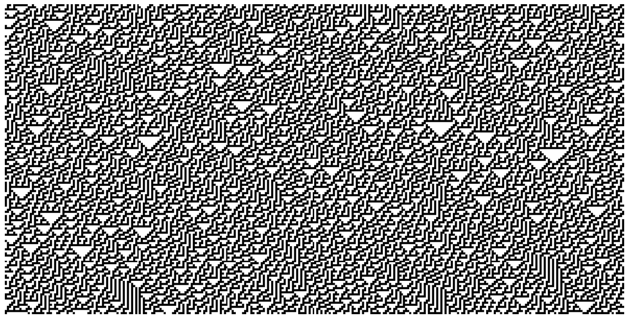

png

学习规则#

在设置好用于生成模拟的代码后，我们现在可以开始探索这些不同规则的属性。沃尔夫勒姆将规则分为四类，如下所述。

def plot_CA_class(rule_list, class_label):
    rng = np.random.RandomState(seed=0)
    fig, axs = plt.subplots(
        1, len(rule_list), figsize=(10, 3.5), constrained_layout=True
    )
    initial = rng.randint(0, 2, 100)

    for i, ax in enumerate(axs.ravel()):
        data = CA_run(initial, 100, rule_list[i])
        ax.set_title(f"Rule {rule_list[i]}")
        ax.matshow(data)
        ax.axis(False)

    fig.suptitle(class_label, fontsize=16)

    return fig, ax

第一类#

快速收敛到均匀状态的元胞自动机

_ = plot_CA_class([4, 32, 172], "Class One")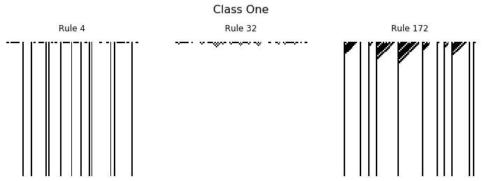

png

第二类#

快速收敛到重复或稳定状态的元胞自动机

_ = plot_CA_class([50, 108, 173], "Class Two")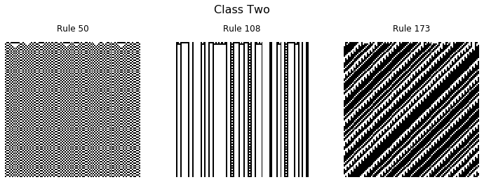

png

第三类#

似乎保持随机状态的元胞自动机

_ = plot_CA_class([60, 106, 150], "Class Three")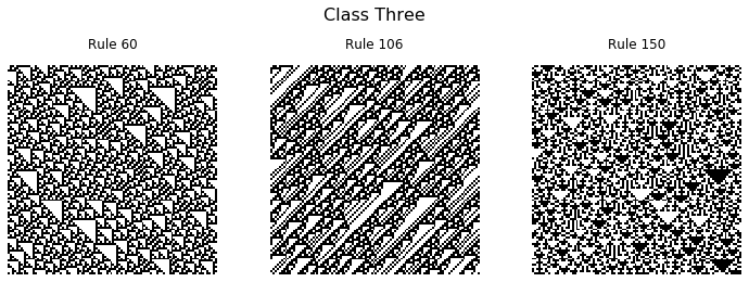

png

第四类#

形成重复或稳定状态区域，但也形成以复杂方式相互作用的结构的元胞自动机。

_ = plot_CA_class([54, 62, 110], "Class Four")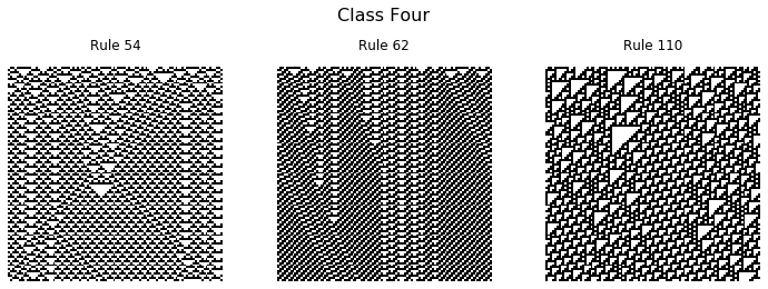

png

令人惊奇的是，从规则 110 中出现的相互作用结构已被证明能够进行通用计算。

在以上所有示例中，都使用了随机初始状态，但另一个有趣的案例是当单个 1 初始化且所有其他值都设置为零时。

initial = np.zeros(300)
initial[300 // 2] = 1
data = CA_run(initial, 150, 30)

fig, ax = plt.subplots(figsize=(10, 5))
ax.matshow(data)
ax.axis(False)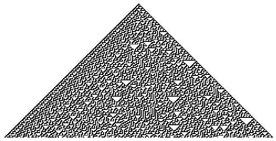

png

对于某些规则，出现的结构以混乱且有趣的方式相互作用。

我希望您喜欢这次对初等元胞自动机世界的简要了解，并受到启发，自己创作一些漂亮的图片。