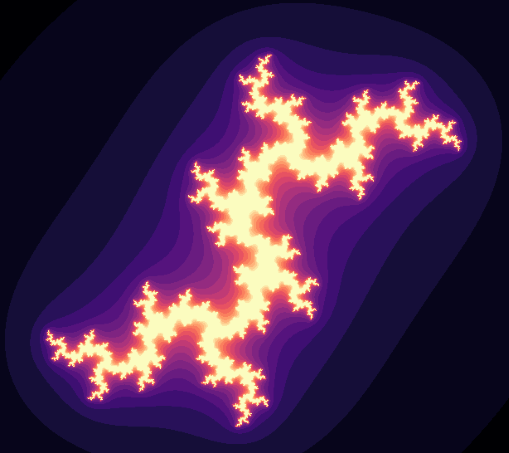
想象一下,不断放大图像,却永远不会失去更精细的细节。这听起来可能很奇怪,但分形的数学概念为我们打开了通往这种错综复杂的无限领域的大门。这种奇特的几何图形无论尺度如何,都表现出相同或相似的图案。我们可以在上面的图片中看到一个分形示例。
由于其特殊性,分形可能看起来很难理解,但事实并非如此。正如分形几何的奠基人之一贝努瓦·曼德尔布罗特在他传奇的TED 演讲中所说
令人惊讶的是,这种几何图形的规则极其简洁。你多次运行这些公式,最终会得到这样的东西(指向一个令人惊叹的图形)
– 贝努瓦·曼德尔布罗特
在本教程博文中,我们将了解如何在 Python 中构建分形,并使用强大的 Matplotlib 动画 API 为其制作动画。首先,我们将通过一个引人入胜的动画演示 曼德尔布罗集的收敛过程。在第二部分,我们将分析 茱莉亚集的一个有趣的特性。敬请期待!
直觉#
我们都对相似性的概念有常识。如果两个物体共享一些共同的图案,我们就说它们彼此相似。
这种概念不仅限于比较两个不同的物体。我们还可以比较同一个物体的不同部分。例如,一片树叶。我们非常清楚,左侧与右侧完全匹配,即树叶是对称的。
在数学中,这种现象被称为自相似性。这意味着给定的对象与其自身的一个较小的部分相似(完全或在某种程度上)。一个值得注意的例子是一个橙色的科赫雪花。它有 6 个凸起,这些凸起本身又各有 3 个子凸起。这些子凸起又有另外 3 个子子凸起。,如下图所示

我们可以无限放大其一部分,并且相同的图案会一遍又一遍地重复出现。这就是分形几何的定义。
曼德尔布罗集动画#
曼德尔布罗集 定义在复数集上。它包含所有复数 c,使得序列 zᵢ₊ᵢ = zᵢ² + c, z₀ = 0 是有界的。这意味着,在一定数量的迭代之后,绝对值不能超过给定的限制。乍一看,它可能显得奇怪且简单,但实际上,它具有一些令人惊叹的特性。
Python 实现非常简单,如下面的代码片段所示
def mandelbrot(x, y, threshold):
    """Calculates whether the number c = x + i*y belongs to the
    Mandelbrot set. In order to belong, the sequence z[i + 1] = z[i]**2 + c
    must not diverge after 'threshold' number of steps. The sequence diverges
    if the absolute value of z[i+1] is greater than 4.

    :param float x: the x component of the initial complex number
    :param float y: the y component of the initial complex number
    :param int threshold: the number of iterations to considered it converged
    """
    # initial conditions
    c = complex(x, y)
    z = complex(0, 0)

    for i in range(threshold):
        z = z**2 + c
        if abs(z) > 4.0:  # it diverged
            return i

    return threshold - 1  # it didn't diverge
如我们所见,我们将迭代的最大次数编码在变量 threshold 中。如果序列在某个迭代处的幅度超过 4,我们将其视为发散(c 不属于该集合),并返回发生这种情况的迭代次数。如果这种情况从未发生(c 属于该集合),我们返回最大迭代次数。
我们可以使用有关序列发散前迭代次数的信息。我们要做的就是将此数字与相对于最大循环次数的颜色相关联。因此,对于复平面网格中的所有复数 c,我们可以根据最大允许迭代次数制作一个关于收敛过程的漂亮动画。
一个特别有趣区域是起始于 实轴 为 -2 和 虚轴 为 -1.5 的 3x3 网格。随着允许迭代次数的增加,我们可以观察收敛过程。这可以通过使用 Matplotlib 的动画 API 很容易地实现,如下面的代码所示
import numpy as np
import matplotlib.pyplot as plt
import matplotlib.animation as animation

x_start, y_start = -2, -1.5  # an interesting region starts here
width, height = 3, 3  # for 3 units up and right
density_per_unit = 250  # how many pixles per unit

# real and imaginary axis
re = np.linspace(x_start, x_start + width, width * density_per_unit)
im = np.linspace(y_start, y_start + height, height * density_per_unit)

fig = plt.figure(figsize=(10, 10))  # instantiate a figure to draw
ax = plt.axes()  # create an axes object


def animate(i):
    ax.clear()  # clear axes object
    ax.set_xticks([], [])  # clear x-axis ticks
    ax.set_yticks([], [])  # clear y-axis ticks

    X = np.empty((len(re), len(im)))  # re-initialize the array-like image
    threshold = round(1.15 ** (i + 1))  # calculate the current threshold

    # iterations for the current threshold
    for i in range(len(re)):
        for j in range(len(im)):
            X[i, j] = mandelbrot(re[i], im[j], threshold)

    # associate colors to the iterations with an interpolation
    img = ax.imshow(X.T, interpolation="bicubic", cmap="magma")
    return [img]


anim = animation.FuncAnimation(fig, animate, frames=45, interval=120, blit=True)
anim.save("mandelbrot.gif", writer="imagemagick")
我们使用 Animation API 中的 FuncAnimation 函数在 Matplotlib 中制作动画。我们需要指定绘制预定义数量的连续 frames 的 figure。一个预定的以毫秒表示的 interval 定义了帧之间的延迟。
在这种情况下,animate 函数起着核心作用,其中输入参数是帧号,从 0 开始。这意味着,为了制作动画,我们总是必须从帧的角度思考。因此,我们使用帧号来计算变量 threshold,它是允许的最大迭代次数。
为了表示我们的网格,我们实例化了两个数组 re 和 im:前者用于 实轴 上的值,后者用于 虚轴 上的值。这两个数组中的元素数量由变量 density_per_unit 定义,该变量定义了每单位步长的样本数量。它越高,我们获得的质量越好,但代价是计算量更大。
现在,根据当前的 threshold,对于我们网格中的每个复数 c,我们计算序列 zᵢ₊ᵢ = zᵢ² + c, z₀ = 0 发散前的迭代次数。我们将其保存在一个最初为空的矩阵 X 中。最后,我们对 X 中的值进行插值,并为其分配来自预先安排的颜色图的颜色。
多次运行 animate 函数后,我们会得到一个令人惊叹的动画,如下所示

茱莉亚集动画#
茱莉亚集 与曼德尔布罗集非常相似。我们不是设置 z₀ = 0 并测试对于某个复数 c = x + i*y,序列 zᵢ₊ᵢ = zᵢ² + c 是否有界,而是稍微切换一下角色。我们为 c 固定一个值,设置一个任意的初始条件 z₀ = x + i*y,并观察序列的收敛情况。Python 实现如下所示
def julia_quadratic(zx, zy, cx, cy, threshold):
    """Calculates whether the number z[0] = zx + i*zy with a constant c = x + i*y
    belongs to the Julia set. In order to belong, the sequence
    z[i + 1] = z[i]**2 + c, must not diverge after 'threshold' number of steps.
    The sequence diverges if the absolute value of z[i+1] is greater than 4.

    :param float zx: the x component of z[0]
    :param float zy: the y component of z[0]
    :param float cx: the x component of the constant c
    :param float cy: the y component of the constant c
    :param int threshold: the number of iterations to considered it converged
    """
    # initial conditions
    z = complex(zx, zy)
    c = complex(cx, cy)

    for i in range(threshold):
        z = z**2 + c
        if abs(z) > 4.0:  # it diverged
            return i

return threshold - 1 # it didn't diverge显然,设置与曼德尔布罗集的实现非常相似。迭代的最大次数表示为 threshold。如果序列的幅度从未大于 4,则数字 z₀ 属于茱莉亚集,反之亦然。
数字 c 使我们能够分析它对序列收敛的影响,前提是最大迭代次数是固定的。对于 c = r cos α + i × r sin α,其中 r=0.7885 且 α ∈ [0, 2π],这是一个有趣的数值范围。
进行这种分析的最佳方法是,随着数字 c 的变化创建动画可视化。这增强了我们对这种抽象现象的视觉感知,并以引人入胜的方式理解它。为此,我们使用 Matplotlib 的动画 API,如下面的代码所示
import numpy as np
import matplotlib.pyplot as plt
import matplotlib.animation as animation

x_start, y_start = -2, -2  # an interesting region starts here
width, height = 4, 4  # for 4 units up and right
density_per_unit = 200  # how many pixles per unit

# real and imaginary axis
re = np.linspace(x_start, x_start + width, width * density_per_unit)
im = np.linspace(y_start, y_start + height, height * density_per_unit)


threshold = 20  # max allowed iterations
frames = 100  # number of frames in the animation

# we represent c as c = r*cos(a) + i*r*sin(a) = r*e^{i*a}
r = 0.7885
a = np.linspace(0, 2 * np.pi, frames)

fig = plt.figure(figsize=(10, 10))  # instantiate a figure to draw
ax = plt.axes()  # create an axes object


def animate(i):
    ax.clear()  # clear axes object
    ax.set_xticks([], [])  # clear x-axis ticks
    ax.set_yticks([], [])  # clear y-axis ticks

    X = np.empty((len(re), len(im)))  # the initial array-like image
    cx, cy = r * np.cos(a[i]), r * np.sin(a[i])  # the initial c number

    # iterations for the given threshold
    for i in range(len(re)):
        for j in range(len(im)):
            X[i, j] = julia_quadratic(re[i], im[j], cx, cy, threshold)

    img = ax.imshow(X.T, interpolation="bicubic", cmap="magma")
    return [img]


anim = animation.FuncAnimation(fig, animate, frames=frames, interval=50, blit=True)
anim.save("julia_set.gif", writer="imagemagick")
animate 函数中的逻辑与前面的示例非常相似。我们根据帧号更新数字 c。在此基础上,我们估计定义的网格中所有复数的收敛情况,前提是允许的迭代次数 threshold 是固定的。与之前一样,我们将结果保存在一个最初为空的矩阵 X 中,并将其与相对于最大迭代次数的颜色相关联。生成的动画如下图所示

总结#
正如我们在本博客中看到的,分形确实是令人难以置信的结构。首先,我们对分形几何进行了总体直观的介绍。然后,我们观察了两种类型的分形:曼德尔布罗集和茱莉亚集。我们在 Python 中实现了它们,并为它们的特性制作了有趣的动画可视化。